Neural Style Transfer - in Pytorch & English
“Style is a simple way
of saying complicated things”
John Cocteau
What is Neural Style Transfer (NST)?
In tech terms:
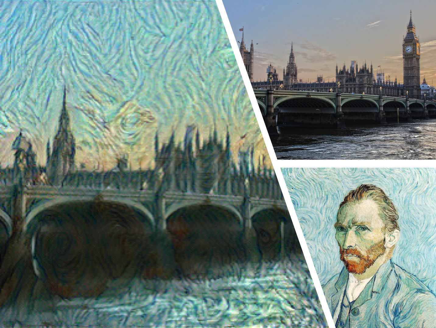
Given 2 input images, generate a third image that has the semantic content of the first image, and the style/texture of the second image.
In dictionary terms:
A way of creating a pastiche - “an artistic work in a style that imitates that of another work, artist, or period."
In pictorial terms:

Individual images taken from original NST paper; annotated by myself
How to do it?
Well if you don’t fancy DIY then this is one part of ML/AI that is already applied in widely consumer available apps like Prisma, DeepArt, Ostagram and Deep Forger. If you want to ‘roll your own’ then keep reading …
In fact, NST has become such a popular application of Neural Networks that a large number of methods have been explored, as can be seen in the taxonomy of NST Techniques below (which will be explained later on, but for now just note the wide array of options highlighted below!)
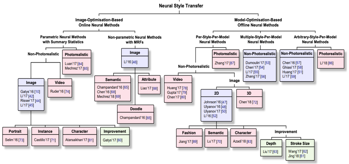
Taxonomy of NST Techniques from “NST: A Review” by Jing et al; Names & dates in each box refer to academic papers outlining the techniques
Though the implementation details, computational efficiency & resulting image quality may differ, the same broad steps need to occur regardless of which NST technique you use:
1. Extract the key features that define the Content you wish to retain in final image
2. Extract the key features that define the Style you wish to apply to that Content
3. Merge the Style features to the Content features in order to generate the new pastiche image
OK, So how can we ‘extract’ style & content?
When I first heard about NST, & of ‘extracting style’ from an image I was deeply suspicious - how can an algorithm define style? Define human creativity & artistic expression after all?… It turns out - pretty easily actually. (Well, extracting sufficient style features to successfully apply them into a pastiche is pretty easy - defining human creativity is a different topic for another time!)
Fortunately Neural Nets, and specifically CNNs, are particularly adept at reducing images to their essential features. If you think of a typical CNN used to classify images – it takes an image & runs it through multiple hidden layers, thereby reducing the image to the key features that best define it, such that it can be classified into a certain category. By running an image through a pre-trained CNN & taking the output at these intermediate (hidden) layers we can thereby access a representation of the key features of that image. Content feature extraction is relatively simple as it is what the given hidden layers already represent; style feature extraction is a little more involved & we need to make some statistical inference in order to extract these features (discussed below). What blew my mind is not only that a CNN can thus reduce artistic style to a set of numerical features, but also that NST is, itself, more of a side-effect of ML. In essence, we do not train a Neural Net to ‘learn’ anything - instead we use the artefacts of a pre-existing trained NN in order to create visually stunning representations.
The seminal paper on NST by Gatys et al. was pre-published in ArXiv.org in 2015 and used VGGNet as the pre-trained CNN to extract image features. I will be using VGG19 for the example Pytorch implementation in this post.
So, what is VGG19 exactly?
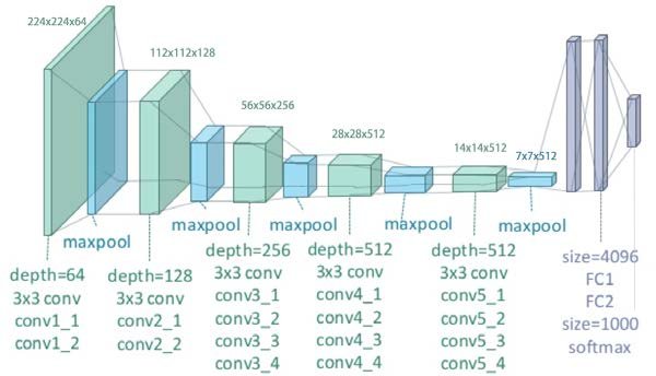
VGG19 is a famous CNN trained on millions of images on ImageNet and capable of classifying images into 1000 categories. (So called VGG after the Oxford University Visual Geometry Group that developed it). The 19 refers to the 19 layer depth of the network – to be precise VGG19 consists of 19 layers with learnable weights: 16 convolutional layers, and 3 fully connected layers. If one counts regularization & pooling layers then there are 47 distinct layers – see below:
So how do we go from VGG19 to the pastiche output?
Taking the original NST paper technique we can compute style and content in the following manner:
1. Create an initial Output Image
2. Calculate Content Loss
3. Calculate Style Loss
4. Update the Output Image to minimize Content & Style Loss, using gradients to directly update pixels
=> Repeat Steps 2-4 until the Output Image is acceptable
A very much simplified overview of these steps is included below - I drew this to help myself understand the high level steps before diving into implementation. (Gatys et al have a more detailed an accurate diagram including Loss Function which I include further below after discussing the details of implementation.)
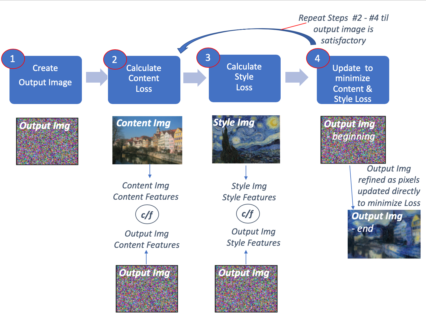
Much simplified view of basic NST process. Again images taken from original NST paper but annotations & overall diagram my own
Each of these steps can be implemented per the below:
1. Create empty image
In the original Gatys paper they initialized the output image to random white noise, noting that starting with either the style or content image skewed the output image toward greater style or content influence.
2. Calculate Content Loss
Extract multiple feature maps from multiple convolutional layers after forward propagating the Content Image (C) and output image (P) through VGGNet. Content Loss is the mean squared error between the feature maps of the content image and of the output image.
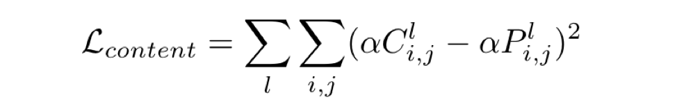
Content Loss: original paper
Content Features: Taking features at intermediate layers; figure source
3. Calculate Style Loss
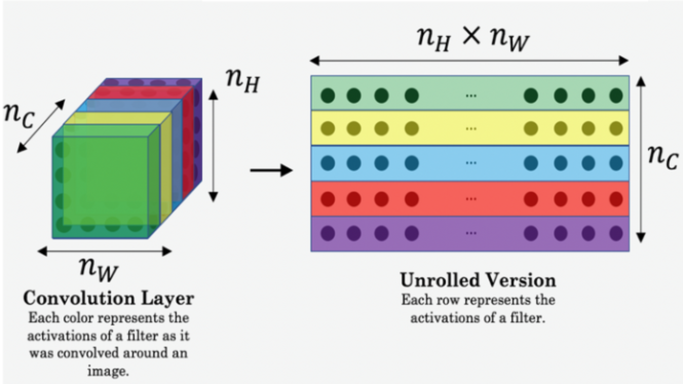
Extract multiple feature maps from multiple convolutional layers after forward propagating the Style Image (S) and Output Image (P) through VGGNet. Style Loss is the mean squared error between the Gram Matrix (Gs) of the style image and the Gram Matrix (Gp) of the Output image. By using the Gram matrices we are calculating feature correlation – essentially the original spatial information of the style image is distributed away and we are left with non-localized information about this image – textures, shapes, weights… those things which, happily, define style!
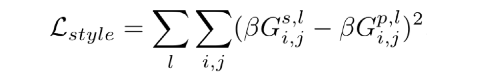
Style Loss: original paper
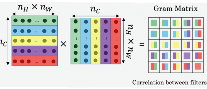
Gram Matrix: columns multiplied by rows show feature correlation; image source
4. Update output image directly to minimize Loss
Our total Loss is equal to the Style Loss and the Content Loss - essentially this represents how far the output image is from the content and style we wish it to exhibit. We also add 2 factors (alpha & beta) to adjust the extent to which we wish to prioritize content vs style in the final output image. In order to improve the output image we directly update its pixels using gradients calculated during backpropagation. Once we have updated the output image, we calculate the new Style & Content Loss & update the output image as required. We continue looping these steps (2-4) until the output image is as we desire (or compute power is used up depending on your access ;-))
Bringing all these steps together we can see from the original paper by Gatys et al how this works:

Enough English - what about the code?
The hardest part of NST (for the original Gatys implementation) is, in my opinion, the conceptual understanding. The code itself is blessedly simple - especially in pytorch - Gram matrices in a single line!? The repo that I found most helpful in getting up and running was that of Yunjey Choi - note that it does not initialize the output image to random noise, but rather the content image. After that the implementation by Justin Johnson (of CS231n fame!) is also great, unsurprisingly. And there is an official Pytorch tutorial here. I have included a snippet of the key code below:
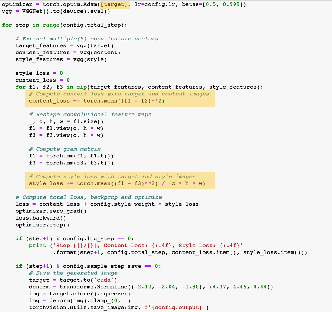
Key pytorch code: note target/output image is fed to the Optimizer as it is the image to be updated; also note Steps #2 & #3 highlighted in yellow
So what about the crazy taxonomy chart from up top?
Returning to the paper by Jing et al. we can now better interpret the taxonomy of NST techniques they outline. Recall (with some annotations now):
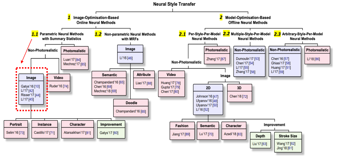
We can see that NST techniques can be split into 2 main categories:
1. Image-Optimisation-Based Online Neural Methods
2. Model-Optimisation-Based Offline Neural Methods
Despite the rather lengthy titles the key difference between these methods is how they treat the extraction of style features. The first ‘online’ methods calculate both the style and content features ‘live’ each time an output image is generated as we did above - indeed the original Gatys method is highlighted in the red dotted bounding box. As a result these methods are expensive computationally and can take a long time to run. The second ‘offline’ methods, create a ‘pre-baked’ style model which remembers style features so that each time a new output image is generated the only ‘new’ features being extracted are those of the Content image. As a result these techniques are faster to run and are how many of the consumer-available NST apps are implemented.
Within the Online methods the first technique (#1.1) uses Gram Matrices to extract style features as we saw. These methods create (qualitatively) attractive output images that minimize the global style and content loss between input and output images. So for content images that are of landscapes they tend to fare very well. However, for fine detailed input (e.g., human portraits) their ability to create meaningful output images can be less impressive. This is because by using summary statistics to infer style and content information they lose semantic information (e.g., do not know which style texture should be used on nose or eyes).
Techniques under #1.2 also work on both style and content images at the same time, but instead of using only summary statistics, they use Markov Random Fields (RMF) in order to more accurately apply styles in their output images. By doing so these methods retain more semantic information and can more accurately apply styles to input content – for instance allowing us to apply the style used for painting eyes in the style image to the eyes in the output image (even if the eyes are in very different sections of the image canvas). Champarndard et al, have a great repo which walks through both their Neural Doodle and Semantic portrait implementation of this sort.
While ‘offline’ techniques under #1 on the Taxonomy produce attractive results and don’t require training data (by using pre-trained CNNs) they suffer from performance issues. Computing the style and content features is very expensive and so creating a single output image can take significant amounts of time, making these techniques unsuitable to user-interative applications for instance.
Within the Offline methods there are 3 main techniques outlined (2.1-2.3). Overall these differ in how generalized their style models are. Recall that offline technique create a ‘pre-baked’ style model - the first group of tecniques (#2.1) create a different model for each style image. (Quite literally there would be a “Van Gough Starry Night” style model vs a “Jackson Pollock Blue Poles” style model for e.g.) This is why you may have encountered NST apps that only allow you to choose from among a number of pre-selected styles to apply to your input image. Techniques 2.2 and 2.3 expand their style models to cover multiple style images and even arbitrary style images (utilizing techniques of batchnorm among others to make them work).
So aren’t you going to end with a picture?
Why yes, yes I will :-) The result of applying Van Gogh style to London Parliament …