Getting to grips with Batch Norms
This week I completed Assignment 2 from the awesome Stanford Cs231n course. This included implementing (among other things) vectorized backpropogation, batch & layer normalization & building a CNN to train CIFAR-10 both in vanilla python and Tensorflow. Implementing batch normalization - particularly the backward pass - was one of the more surprising parts of the assignment, so I thought I would write about it here.
What is it?
Batch Normalization is a technique to improve learning in neural networks by normalizing the distribution of each input feature, of each layer, across each mini-batch of training data to a set mean and variance. It is most common to normalize to a unit Gaussian (or, in high school math terms a ‘normal distribution’!) of zero mean and variance of 1 - N(0, 1).
What is the problem it addresses? (AKA: Why Bother)
Internal covariate shift - in the intermediate layers of a neural network the distribution of activations (outputs from each layer) are constantly shifting. This slows down the training of the network as it needs to learn to adapt to each new distribution in every single training step. Batch normalization reduces the amount by which the hidden unit values shift around & so improves efficiency.
Moreover it allows you to use, on average, higher learning rates as batch norm ensures activations don’t become too high or low. If that weren’t enough, it always provides a regularization effect which means that nets are, overall, less sensitive to poor initialization of weights and require less dropout or other regularization techniques. As the authors of the seminal paper put it:
Applied to a state-of-the-art image classification model, Batch Normalization achieves the same accuracy with 14 times fewer training steps, and beats the original model by a significant margin. Using an ensemble of batch-normalized networks, we improve upon the best published result on ImageNet classification: reaching 4.9% top-5 validation error (and 4.8% test error), exceeding the accuracy of human raters.
Sergey Ioffe, Christian Szegedy in original batch norm paper
N.B. The original paper is written in a clear and straightforward manner so I highly recommend it, even if academic papers aren’t usually your cup of tea.
OK, so - batch norm always works then?
If batches become very small or do not consist of independent samples then the batch means and variance may become poor approximations of the overall dataset. As such, batch normalization has been shown to perform poorly with very small batches. But broadly speaking it is a great place to start.
OK … But how do I implement it?
It is pretty simple in theory (and in practice on the forward pass - more on that later). Essentially wherever we want to implement batch norm we insert a batch norm layer into the network. The batch norm layer then does the following calculations as outlined in the image below (from the original paper, annotations mine):
Calculate the mean & variance of the input to the layer
Normalize these inputs using the statistics calculated above
Scale and shift with a linear function in order to obtain the output of the layer
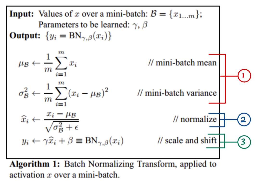
From original Batch Norm paper, handwriting my own
#3 the “Scale & Shift” function is really interesting. This essentially allows the network to ‘undo’ the effect of batch norm if it finds, in training, that simply using the original un-normalized input works better for accuracy. I found that viewing this in a very simplified computational graph helped me most with seeing this clearly:
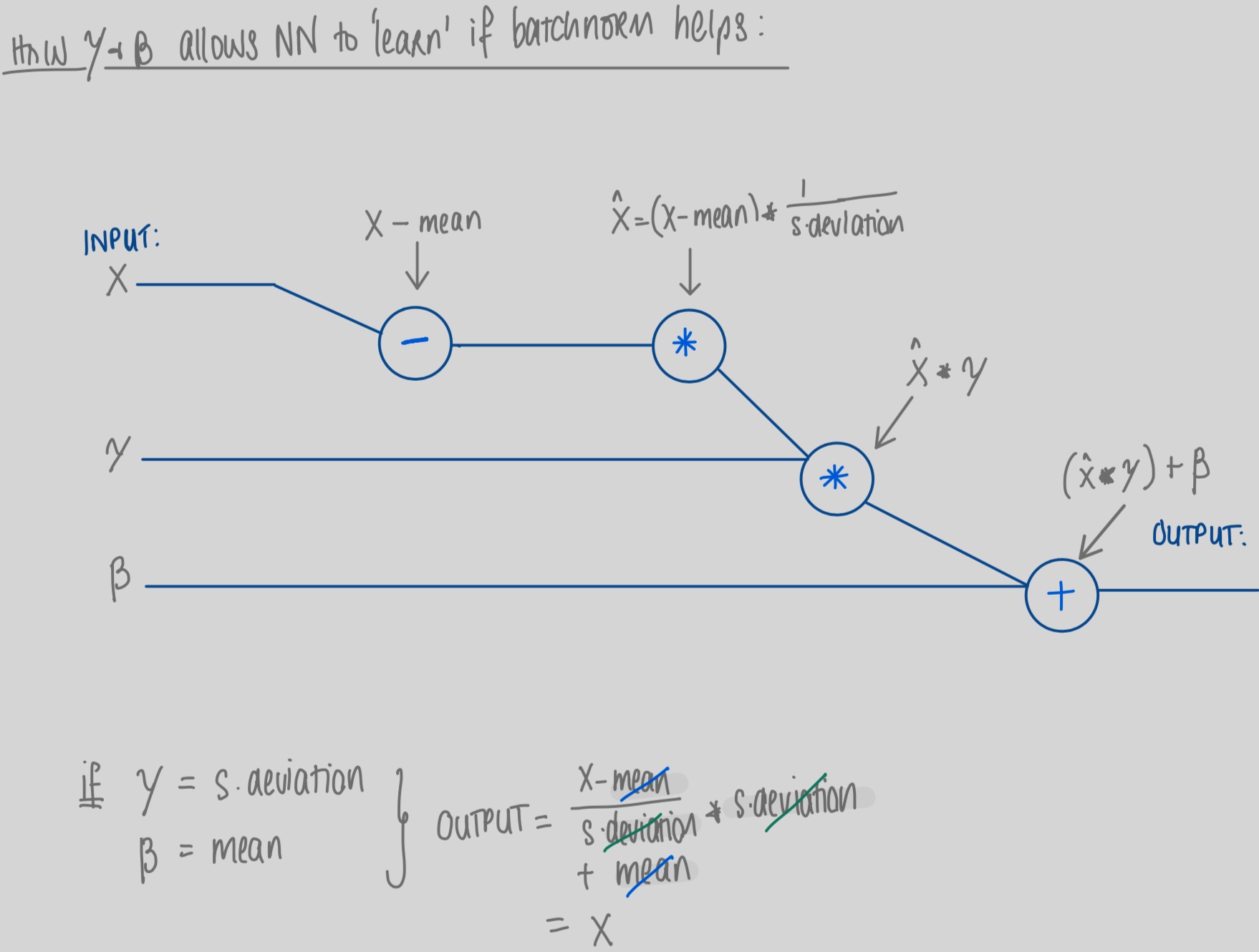
Gamma & Beta are learnable parameters. In the image above we can see a simplified view of a forward pass where inputs are normalized by subtracting the mean and dividing by the standard deviation. The network then multiplies this output by the parameter gamma and adds the parameter beta in order to calculate the output for the batch norm layer. It can thus be seen clearly how a network could learn to ‘undo’ normalization if it was not helping accuracy in the network. (NB. Inputs X are a tensor and Gamma & Beta vectors; for simplicity the graph is in general terms and does not detail summation across dimensions).
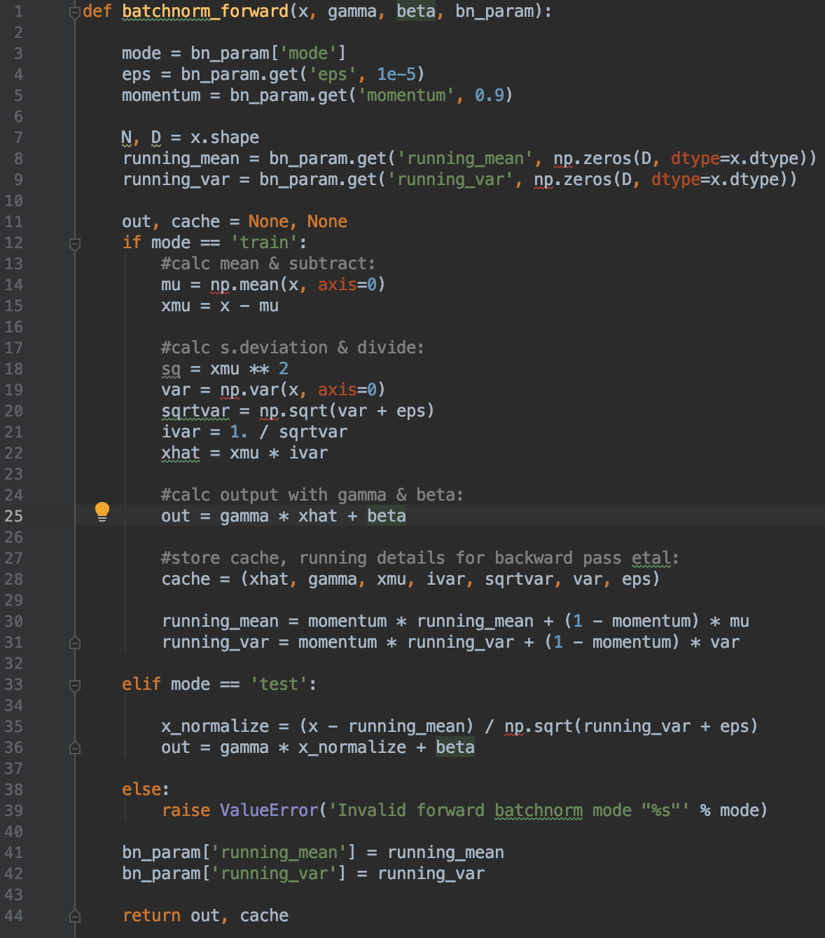
It also shows a simple way to think about implementing a vanilla batch norm forward pass as seen in lines 13-35 of the training block below:
Is implementing the backward pass as easy?
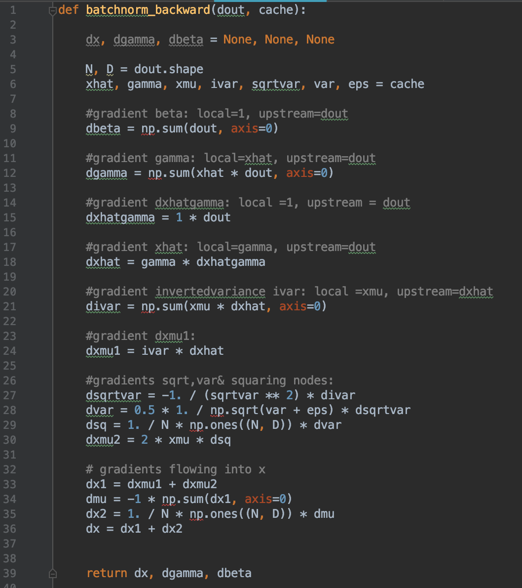
Not really… but it’s not that hard ;-) Again thinking in terms of small steps in a computational graph helped me a lot in calculating the gradients piece by piece. This is by no means the most elegant or efficient implementation of backprop! But for understanding how backprop works I really valued breaking down the function into small steps in a computational graph and backing into the key gradients.
In my hand-drawn diagram below you can see the names of each intermediate step from the forward pass in blue, and the gradients from the backward pass in red (e.g., the first multiplication gate is xhat on the forward pass, and the gradient on the backward pass is dxhat).
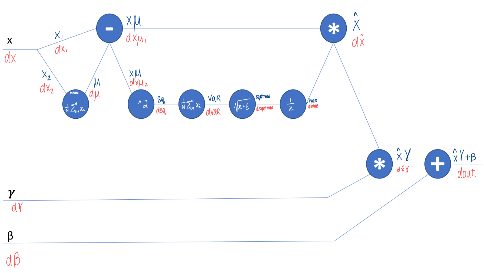
Based on breaking down the batchnorm into these small steps, a vanilla python implementation can be seen below. For clarity I have calculated all gradients in the form of: local gradient * upstream gradient to reflect the chain rule and make comprehension easier. For example in the first multiplication node xhat, the gradient dxhat is calculated as the local gradient (gamma) * the upstream gradient relative to overall loss (dout).
So …. what?
Overall I feel like the lessons for me this week were:
Computational graphs are powerful & Andrej Karpathy lectures are phenomenal
Batchnorm is something I will be implementing more often than not in my networks
I will, however, be using Tensorflow/Pytorch to do so ;-)
I am eternally grateful for Andrej Karpathy & Frederik Kratzert for their clear blog posts as I tackled this challenge!